My quest for the Instrument Rating has lead me to learn more about weather, pretty scary huh? I have been fascinated with the Skew T diagrams since I first read about them on the Pilots of America Forum. Multiple posts and good info shared by Scott Dennstaedt, CFII & Former NWS Meteorologist,Nationwide Cessna 350/400 Factory Instructor, IFR Magazine Contributing Editor Writer for Plane & Pilot, Pilot Journal and Twin & Turbine.
Scott offers a training course through Chesapeake Aviation Training and the link will provide a glimpse of the Skew T. I spent the day shooting approaches online since I could not get out of Wilmington this morning in order to make my 7am lesson. It sure would have been nice to get some actual in the soup but as they say, no IFR ticket,no wash. Between approaches I scoured the Internet reading about weather and the Skew T. I think I will be sending for Scott's training CD.
Below, I listed the link and info that Jeff Haby provided on my subject of the day. Sit back, read along and see what you think about this added weather info that is available for us to digest.
SKEW-T BASICS by Meteorologist Jeff Haby
The Skew-T Log-P offers an almost instantaneous snapshot of the atmosphere from the surface to about the 100 millibar level. The advantages and disadvantages of the Skew-T are given below:
Why do we need Skew-T Log-P diagrams?
Can assess the (in)stability of the atmosphere
Can see weather elements at every layer in the atmosphere
Determine cap strength, convective temperature, forecasting temperatures,
determine character of severe weather
This is the data used to produce the synoptic scale forecast models
What are some disadvantages of Skew-T's?
Only available twice a day (00Z and 12Z)
Character of weather can change dramatically between soundings
Sounding does not give a true vertical dimension since wind blows balloon downstream
Sounding does not give true instantaneous measurements since it takes several minutes to travel from the surface to the upper troposphere.
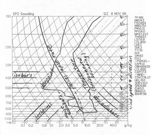
Below are all the basics lines that make up the Skew-T
Isobars-- Lines of equal pressure. They run horizontally from left to right and are labeled on the left side of the diagram. Pressure is given in increments of 100 mb and ranges from 1050 to 100 mb. Notice the spacing between isobars increases in the vertical (thus the name Log P).
Isotherms- Lines of equal temperature. They run from the southwest to the northeast (thus the name skew) across the diagram and are SOLID. Increment are given for every 10 degrees in units of Celsius. They are labeled at the bottom of the diagram.
Saturation mixing ratio lines- Lines of equal mixing ratio (mass of water vapor divided by mass of dry air -- grams per kilogram) These lines run from the southwest to the northeast and are DASHED. They are labeled on the bottom of the diagram.
Wind barbs- Wind speed and direction given for each plotted barb. Plotted on the right of the diagram.
Dry adiabatic lapse rate- Rate of cooling (10 degrees Celsius per kilometer) of a rising unsaturated parcel of air. These lines slope from the southeast to the northwest and are SOLID. Lines gradually arc to the North with height.
Moist adiabatic lapse rate-- Rate of cooling (depends on moisture content of air) of a rising saturated parcel of air. These lines slope from the south toward the northwest. The MALR increases with height since cold air has less moisture content than warm air.
Environmental sounding-- Same as the actual measured temperatures in the atmosphere. This is the jagged line running south to north on the diagram. This line is always to the right of the dewpoint plot.
Dewpoint plot- This is the jagged line running south to north. It is the vertical plot of dewpoint temperature. This line is always to the left of the environmental sounding.
Parcel lapse rate-- The temperature path a parcel would take if raised from the Planetary Boundary Layer. The lapse rate follows the DALR until saturation, then follows the MALR. This line is used to calculate the LI, CAPE, CINH, and other thermodynamic indices.
Below is an example diagram showing the lines of the Skew-T Log-P diagram
Scott offers a training course through Chesapeake Aviation Training and the link will provide a glimpse of the Skew T. I spent the day shooting approaches online since I could not get out of Wilmington this morning in order to make my 7am lesson. It sure would have been nice to get some actual in the soup but as they say, no IFR ticket,no wash. Between approaches I scoured the Internet reading about weather and the Skew T. I think I will be sending for Scott's training CD.
Below, I listed the link and info that Jeff Haby provided on my subject of the day. Sit back, read along and see what you think about this added weather info that is available for us to digest.
SKEW-T BASICS by Meteorologist Jeff Haby
The Skew-T Log-P offers an almost instantaneous snapshot of the atmosphere from the surface to about the 100 millibar level. The advantages and disadvantages of the Skew-T are given below:
Why do we need Skew-T Log-P diagrams?
Can assess the (in)stability of the atmosphere
Can see weather elements at every layer in the atmosphere
Determine cap strength, convective temperature, forecasting temperatures,
determine character of severe weather
This is the data used to produce the synoptic scale forecast models
What are some disadvantages of Skew-T's?
Only available twice a day (00Z and 12Z)
Character of weather can change dramatically between soundings
Sounding does not give a true vertical dimension since wind blows balloon downstream
Sounding does not give true instantaneous measurements since it takes several minutes to travel from the surface to the upper troposphere.
Below are all the basics lines that make up the Skew-T
Isobars-- Lines of equal pressure. They run horizontally from left to right and are labeled on the left side of the diagram. Pressure is given in increments of 100 mb and ranges from 1050 to 100 mb. Notice the spacing between isobars increases in the vertical (thus the name Log P).
Isotherms- Lines of equal temperature. They run from the southwest to the northeast (thus the name skew) across the diagram and are SOLID. Increment are given for every 10 degrees in units of Celsius. They are labeled at the bottom of the diagram.
Saturation mixing ratio lines- Lines of equal mixing ratio (mass of water vapor divided by mass of dry air -- grams per kilogram) These lines run from the southwest to the northeast and are DASHED. They are labeled on the bottom of the diagram.
Wind barbs- Wind speed and direction given for each plotted barb. Plotted on the right of the diagram.
Dry adiabatic lapse rate- Rate of cooling (10 degrees Celsius per kilometer) of a rising unsaturated parcel of air. These lines slope from the southeast to the northwest and are SOLID. Lines gradually arc to the North with height.
Moist adiabatic lapse rate-- Rate of cooling (depends on moisture content of air) of a rising saturated parcel of air. These lines slope from the south toward the northwest. The MALR increases with height since cold air has less moisture content than warm air.
Environmental sounding-- Same as the actual measured temperatures in the atmosphere. This is the jagged line running south to north on the diagram. This line is always to the right of the dewpoint plot.
Dewpoint plot- This is the jagged line running south to north. It is the vertical plot of dewpoint temperature. This line is always to the left of the environmental sounding.
Parcel lapse rate-- The temperature path a parcel would take if raised from the Planetary Boundary Layer. The lapse rate follows the DALR until saturation, then follows the MALR. This line is used to calculate the LI, CAPE, CINH, and other thermodynamic indices.
Below is an example diagram showing the lines of the Skew-T Log-P diagram
1 comment:
Good stuff Gary. I'm also interested in learning more about the Skew-T diagram. It's been on my to-do list for a few months now. ;)
Let us know what you think of Scott's course if you take it.
Post a Comment